Short introduction to the spectral sequence
Theory
- Spectral Lines
- Wavelenght Units
Why so many different spectra?
Since 1860-1880 father Angelo Secchi, Huggins, Vogel and others discovered that
the great majority of the stars spectra can be classified in few classes and that peculiar
spectra concern only a small number of stars.
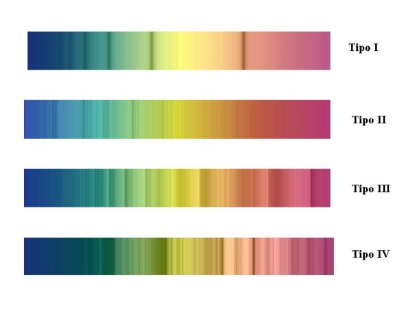
As an example of early classification scheme, we describe Secchi's classification that was
based on 4 classes. In the first class Secchi included all the
blue-white stars (like Vega or
Rigel) that show only few lines.
In the second class were included all the yellow stars like the sun, Arcturus and Capella
that show many narrow lines.
In the third class were included the red-orange stars with many narrow lines and some absorption
bands with the head toward the blue (like Betelgeuse
or Mira Ceti)).
In the fourth class were included the ruby-red stars with absorption bands with the head toward
the red (nowadays we call them "carbon stars" like 19
Psc ).
|
|
Picture 1: Tipical star spectra as they could be observed with prism spectrographs
that were used by astronomers of the eigthteenth century. Dark absorption lines and bands
overlap to the bright continuum. From the top the spectra are Vega, sun,
r Per, 19 Piscium.
|
In order to understand a stellar spectrum it is necessary to know at least some of the
more common interactions between light and matter.
Those of interest here are blackbody emission and atomic absorbtion and emission.
The emission spectrum of heated bodies ("Black Body" spectrum)
Every heated body produces a continuum spectrum of radiation that depends (with more
or less approximation) only on its temperature.
As an example, a heated metallic rod shines with a dark red color when it is relatively cold but
its color become yellower and brighter as the temperature increases and reaches fusion (1500 K).
This behaviour of the metal rod is close to the behaviour of an ideal black body.
A black body is able to re-absorb all the light it produces and thus a thermal equilibrium is
established between the matter and the radiation.
The thermal energy stored in the matter is transferred to radiation and vice-versa. So if
the matter is hotter, more energetic photons will reach equilibrium with the matter and the
radiation that eventually can escape has a shorter wavelenght (remember that a photon brings
an energy h n and thus is blue shifted.
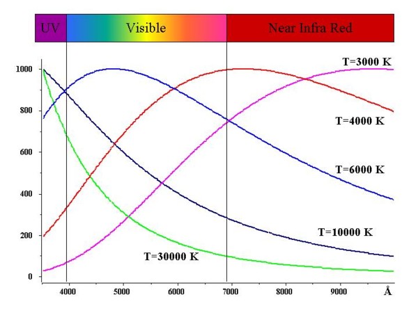
The picture 2 shows the spectral distribution emitted by black bodies of different temperature.
|
|
Picture 2: Density of energy emitted per unit surface (normalized at maximum) of 5 black bodies
heated at different temperatures: 30000, 10000, 6000, 4000, 3000 K.
Note that the maximum of radiation lies outside the visible range for the higher and lower
temperatures.
|
Black body emission is submitted to two very simple physical laws.
Wien law states that the wavelenght of the emission maximum is
lmax
[mm]=2950/T where T is in degrees Kelvin.
The Stefan-Boltzmann law states that the overall radiation emitted per unit surface by a black
body is proportional to the fourth power of the temperature.
This second law has a deep impact on the luminosity of stars. Infact a star with surface
temperature of 10'000 K is 16 times brighter than a 5000 K star of equal radius.
The stellar photospere behaves pretty like a black body and its emission explains the
continuum that can be observed in the stellar spectra. From the maximum of emission the
temperature of the star can be deduced.
The complete formula, obtained by Planck for the spectral density of energy emitted per unit
surface is E=(c1/l5)/[e(c2/KT)
] where T is expressed in Kelvin degrees, l in cm,
c1=3.7419 x 10⁻⁵, c2=1.4288 cm K.
Emission and absorbtion spectra of atoms and molecules
Many materials (for example the rarefied gases of the stellar atmospheres) do not behave like
a black body because they are mainly transparent and can absorbe in correspondance of few
wavelenghts.
This happens because only particular orbits are allowed for electrons inside atoms.
These orbits have fixed energies and when an electron jumps from one orbit to another a fixed
amount of energy (and thus light at a particular frequency) is absorbed or emitted.
The energy of the orbits is unique for each type of atom and thus unique are the wavelenghts of
the emitted lines.
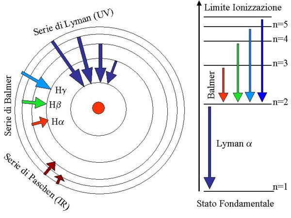
In the picture 3 is described the hydrogen atom, that is the more simple (only one proton and
one electron) and in the same time the more abundant in the universe.
|
Picture 3: Permitted orbits inside the hydrogen atom are identified by the quantum number
n=1,2,3,4, ... that correspond to energetic levels (diagram of the right side) of the atom.
The energetic levels representation is the only used for the more complex atoms.
All the electron transitions that end on the lower orbit (fundamental state) belong to the
Lyman series that can be observed in the UV.
All transitions that ends on the second orbit (n=2) form the Balmer series, in the visible.
The wavelenghts in Angstrom of the Balmer lines are given by the formula:
911,4/(1/4-1/n2) where n=3 for Ha, n=4 for
Hb etc...
Transitions that ends on the n=3 orbit belongs to the Paschen series that can be observed (for
example in the spectrum of novae) between 8203 and 18750 Ĺ.
|
All other atoms have a higher nuber of electrons and thus an increasing number of allowed
orbits and spectral lines.
Iron, for example, has 26 electrons that produce thousands of lines. Many of them can be observed
in the stellar spectra.
Emission lines are produced when an electron jumps from an upper orbit to an inner one.
Absorption lines are due to a jump from an inner orbit to an upper one.
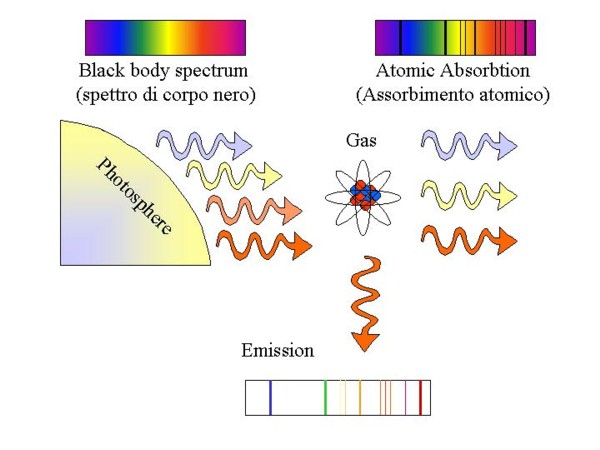
We have now all the elements to understand, at least qualitatively, the origin of stellar
spectra. The continuum emitted from the photosphere is selectively absorbed at those
wavelenghts that correspond to the energetic jumps of the atoms in the stellar atmosphere.
|
Picture 4: Absorption and emission spectrum from the transparent gas that is surrounding a
star. In order to produce an emission spectrum, the UV photons from the star excite the atoms
of the gas that relax to lower energy state emitting photons with energy that equals the energetic
jumps of the emitting atoms.
|
Population of atomic levels and ions production. The role of temperature
As we have already seen, the surface temperature of a star can be obtained from the maximum of its
continuum black body emission.
Temperature changes the population of electronic levels, thus the intensity of lines that generate
from the levels.
The difference among stellar spectra is due manly to this effect.
Let's see in some more details how this works.
Electronic levels population follows the Maxwell-Boltzmann statistics. In M-B statistics for
two levels with energy E1 and E2, the ratio of the two populations is
N1/N2=(g1/g2)xe(E1-E2)/kT, where g1 and g2 are the statistical weights
(magnetic degeneration) of the two levels and k is the Boltzmann constant.
If the energy E is expressed in eV, the Boltzmann constant is 8.617x 10⁻⁵ eV/°K.
Some time the energy of the electronic levels is expressed in cm-1. Conversion in eV
can be done dividing by 8065.541 cm-1/eV.
As an example, let's take the n=1 (foundamental and the lower one) and n=2 levels of the hydrogen
atom. The difference in energy (E1-E2) between these 2 states is 10,2 eV.
When the temperature is close to zero K, all the hydrogen atoms have their electron at the
lower level (n=1) and thus the absorbtion spectrum will contain only the Lyman series.
When temperature grows, more and more electrons jump on the n=2 and higher orbits.
Multiplicity of the n=1 state (1s) is 2 while for n=2 (2s+2p orbitals) multiplicity is 2+6=8.
When the temperature reaches 10'000 K the Botzmann law says that 0,04% of the electrons are now
on the n=2 orbit and in the spectrum will appear also the Balmer series.
Increasing even more the temperature, the electron can jump outside the atom and ionisation
of the hydrogen atoms occurs. Whithout electrons, the hydrogen atom loses its capability of
absorbing light. Thus in the hottest stars, the hydrogen spectrum disappears.
Also metals behave like hydrogen and when the temperature increase, they start to loose
their outer electrons. The remaining inner electrons produce transitions that lie in the UV and
thus lines due to metals also disappear in the hottest stars.
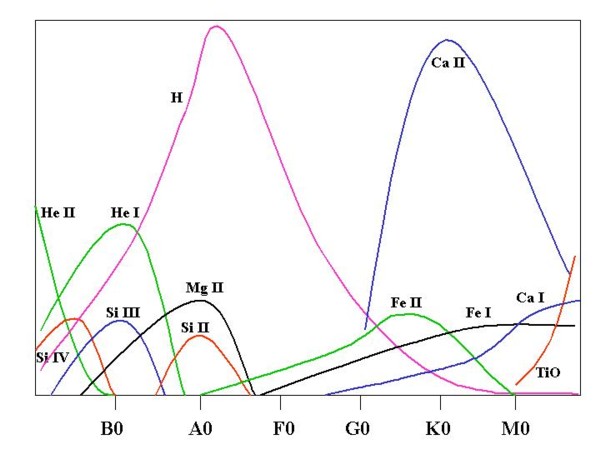
Picture 5 shows the intensity of the lines produced by particular ions as a function of
temperature (or spectral class, that is almost the same).
In the astronomical spectra, lines produced by ions are identified with the symbol of the element
followed by roman numbers that indicate the state of ionisation. As an example, "Fe I" means
neutral Iron, "Fe II" means Iron that has lost one electron, "Fe III" means Iron that has lost
2 electrons and so on.
|
Picture 5: Line intensity for some important ions and atoms along the spectral sequence.
He and highly ionized elements dominate the spectra in the hottests classes.
Hydrogen Balmer series reaches maximum intensity at A2 while in colder stars become more
and more important the contribution of neutral metals.
|
In the spectrum of the hottest stars, the only strong lines are due to neutral and ionized Helium
whose ionisation energy is 24.6 eV, the highest among all elements, almost double if compared
to hydrogen (13,6 eV) and three times that of Iron (7,9 eV).
Once again we find that temperature is the main parameter that makes spectra change even if
the chemical composition of stellar atmospheres is almost identical from star to star.
Miss Cannon in the first years of the 20th century was the first to understand this temperature
dependence as deduced from the observation of 225'000 star spectra.
Her spectral classification, based on the O-B-A-F-G-K-M classes is ordered from higher to lower
temperatures while the previous Harward classification A-B-C-D-E-F-G ... was based on the
strenght of hydrogen lines.
Here is a table of temperatures related to the spectral classes O -
B -
A -
F -
G -
K -
M .
| Class | Temperature (K) | Spectral Features |
| O | +28'000 | He ed He+ per le piu' calde |
| B | 28'000 - 12000 | He, Balmer, Si III, O II |
| A | 12'000 - 7'000 | serie di Balmer molto intensa, deboli Mg II e Fe II |
| F | 7'200 - 5'500 | Ca II, Balmer, Fe II, Ti II, Y II, Sr II |
| G | 6'000 - 4'500 | Ca II, Balmer, metalli neutri (intensi NaI, Fe I) |
| K | 4'700 - 3'000 | Ca II, prime molecole (CN, CH), metalli neutri (Na I, Fe I, CaI) |
| M | < 3'300 | metalli neutri (Ca I, Na I, Fe I), molecole CH, CN, TiO |
The spectral classification that is used nowadays is a refinement, proposed in 1943 by
Morgan, Keenan, Kellman (and thus sometimes indicated as MKK) of the original
Cannon classes.
Each spectral class is divided into numbered subclasses. As an example K class is divided
into K1, K2, K3, K4, K5 from the hottest to the coldest.
Giant and Dwarfs: HR diagram
Compared to the Harward classification, the modern MKK scheme adds a second parameter
that indicates the luminosity class of the star.
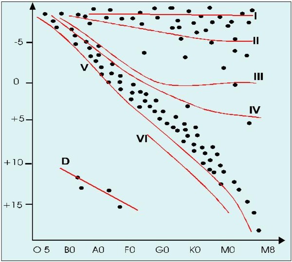
As was discovered by Herzprung and Russel in 1914, for a given temperature (and thus for the
same spectral class) can exist dwarfs, giants and super-giants stars. This is shown in the HR
plot in the picture 6.
Supergiants are indicated with the roman number I, the luminous giants with II, the giants with
III, the sub-giants with IV and the main sequence dwarfs with V.
As an example, the complete spectral classification of the sun is G2 V.
There is also a weakly populated luminosity class IV that collect main sequence star of
population II that have a low metallic content.
The luminosity class D includes the white dwarfs
.
The I supergiants class is further divided into Ia and Ib, where Ia is given to exceptionally
bright stars.
|
Picture 6: HR plot that shows the position of stars in fuction of their temperature
(spectral class) and luminosity. For a same temperature (and thus for the same spectral class) it is possible to
find stars of a very different brightness.
Brightness is expressed in terms of absolute luminosities, ie the magnitude at a standard
distance of 10 parsec (32,6 anni luce).
|
We can make many useful considerations for the spectroscopist on the HR plot.
If we consider the main sequence stars we observe that an M dwarf is 10 to 15 mag less bright
than a G dwarf like our sun. Few red dwarfs will be easily observable (and none infact is visible
to the naked eye), even if they are probably very abundant in the galaxy.
The same can be said for the white dwarfs.
Even greater is the brightness difference between M dwarfs and supergiants. Up to 30 mag!
As we know that for an M giant and dwarf the temperature is approximately the same (and
thus they have the same black body emission per unit surface), the supergiants
must have an enormous diameter in order to be so bright.
Infact stars like Betelgeuse or Antares are comparable to Jupiter orbit.
A consequence of these huge dimensions is that the density is extremely low.
The luminosity gap reduces progressively going up in the main sequence and by type O there is
almost no difference between a dwarf and a giant.
Even if the O, B, A stars are relatively uncommon, due to their high brightness, they are well
represented among constellations.
| Class | Mv. dwarfs | Mv. giants | Dwarf example | Giant example |
| O | ---- | < -4 | ---- | z Ori |
| B | -4 a +2 | -5 | Spica | Rigel |
| A | +2 | -6 | Vega | Deneb |
| F | +4 | -7 | p3 Ori | a Per |
| G | +5 | -7 | Sole, 9 Ceti, 16 Cyg, a Cen | 9 Peg |
| K | +8 | -7 | 61 Cyg | e Peg |
| M | +13 | -5 | 40 Eri C | Betelgeuse |
Spectral differences between dwarfs and giants. The effect of density. The Saha law
How is it possible from its spectrum to say that a star is a dwarf and not a giant or supergiant
of the same spectral class?
The answer is: Measuring the density of the star atmosphere from the line profile.
The giant and supergiant stars infact are much bigger but with lower density than dwarfs and
a low pressure gas produces sharper lines.
There are also other differences. At the same temperature but at a lower density, ionisation
is enhanced because once an atom has lost an electron, it is difficult in a low pressure
environment to find out another electron for recombination.
In the giants it is thus observed a higher intensity of the ions lines compared to dwarfs of the
same spctral class.
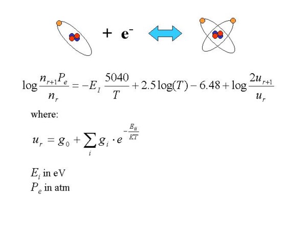
It is possible to calculate the ratio between neutral atoms population and ions population
considering the equilibrium Ion+electron=Neutral Atom .
This equilibrium depends on the Boltzmann Statistics (and thus from the temperature and energy of
the excited states) but also from the density. This result was obtained by Saha and the formula
that gives the ratios of ions populations is called Saha formula.
|
Picture 7: The mathematical formulation of the Saha law that allows to calculate
(recursively) the number of atoms that are in a certain state of ionisation.
These ratios depend on the ionisation energies (Ei) of the atoms, on the temperature (T)
and on the electronic pressure (Pe).
|
The higher intensity of the lines of the ionized elements in the giants has brought
to classify giants in subclasses somewhat hotter than the corresponding dwarfs.
Between a giant and a dwarf of equal spectral class there can be some undreds of K degrees of
difference.
Typical electronic pressures for main sequence stars are between 10-6
e 10-4 atm and for the giants some order of magnitude lower.
Very hot and very cold stars. Chemically peculiar stars
Both the beginning and the end of the spectral sequence collect stars whose spectra cannot
be explained only with density and temperature.
In these stars, evolution has produced also some chemical differences.
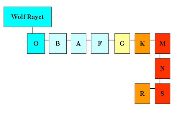
On the side of the hot stars we find the Wolf-Rayet
stars , with broad emission lines, due to the inner layers of the star that are
brought to surface by the very strong stellar winds.
From the side of the cold M and K stars we encounter the
"carbon stars" . In these stars, the high carbon content reduces the amount of
oxygen in the atmosphere and the TiO bands that are typical of M stars cannot form any more.
Instead, we can observe the Swan bands due to C2 and sometimes the ZrO bands.
Carbon stars are classified N if their temperature is comparable to the temperature of M stars,
while they are lassified as R if the temperature is in the range of K stars temperature.
Picture 8 shows the full spectral sequence, comprehensive of peculiar strs classes.
|
Figura 8: La sequenza spettrale completa
|
Vai a :
Spectral lines
- Wavelenght units
|
|